Loading and viewing data 🦆⚽
- Check out the GitHub repo
- See the data in Google sheets format here.
Now that we have created our source files, we need to upload them into a DuckDB database, verify the data and re-format to create our final analysis-ready tables. DuckDB makes loading data very easy and its schema feature is very convenient for organasing tables and other database objects.
Before we start
I am assuming the following:
- You have installed DuckDB - to verify execute
which duckdbfrom your terminal. If you get nothing back, then DuckDB is not installed or is not in your executables path. - You have checked out the code from the GitHub repo
Getting started
We now have our files ready for loading into DuckDB. Our DuckDB database file is simply called epl.ddb. To load our data, we first need to create a DuckDB database which we can do very easliy by changing to the db_files directory and executing the command:
duckdb epl.ddb
Executing this command now lands us in the duckdb command line client and you should see the D prompt. You can now start issuing commands that the client will execute against the DuckDB database file. If you have used the SQLite sqlite3 client it will feel very familiar. However, even if you are new to it, it is not difficult to learn. The most important point to remember is that it takes two types of commands:
-
Dot commands: so called because they begind with a period (.). They are used to perform tasks such as listing all objects of a certain type such as tables, importing/exporting data and for setting certain DuckDB variables. From the client, try
.helpto see the options. Note that nothing, not even white space can precede the dot and the dot command is not terminated by a semicolon. -
SQL commands: These are standard DuckDB SQL commands and they are not preceded by a dot but are terminated by a semi-colon. We will see loads of these throughout for creating tables, selecting/updating/deleting data and do on. When you enter a command in the DuckDB shell and hit return without the the terminating semi-colon, you will see the secondary prompt, ‣ whiich indicates that the client is waiting for additional input.
If you exit the DuckDB client by issuing one of the dot commands .q or .quit without creating any objects, the database file will not be saved. If you create any content, even an empty table, the file named epl.ddb will be created and saved.
Importing our first file
We cannot do much with the data in DuckDB until we import it but first we can have a look at it before we do a full import.
Explore before loading
We are going to import the file seasons_1993_2023.tsv which we generated using a shell script in the previous chapter. Before we import the file, we can take a “sneak peak” at it by executing the following command in the DuckDB client at the D prompt:
SELECT * FROM '../output_data/seasons_1993_2023.tsv' LIMIT 5;
You should see something that looks like the following in your teminal:
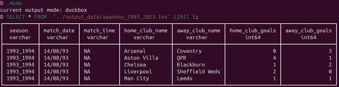
By default the output appears in what DuckDB calls current output mode: duckbox. You can verify this by issuing the .mode dot command. We will see later how to change this mode to customise outputs from queries.
Like the Unix head command, the SQL query above shows all columns for the file. However, unlike head, by default it recognises the first row as the column names. To get the equivalent output from head, you woud need to execute head -6 ../output_data/seasons_1993_2023.tsv. The SQL query output also informs us that there are seven columns and it has assigned data types to those columns. The data types are DuckDB guesses based on available data and we are free to change column data types to other compatible data types for particular columns which we will do later.
The SQL command above is interesting because DuckDB is allowing to to select data directly from a file. This is a novel and very useful feature of DuckDB. It is one of its many very convenient features and really useful for exploring data.
Import the file
You can import files in the same way as in SQLite using the .import FILE TABLE command but DuckDB has added easier ways to do this which we will exploit here.
Schemas
Unlike SQLite but like PostgreSQL, DuckDB provides a schemas which are convenient for dividing your database into logical units. Every DuckDB database has a default schema called main; in PostgreSQL the equivalent default schema is called public. They are somewhat like namespaces and allow us to group similar objects together. A common pattern in database programming is to load new and unverified data into a staging area where it can be stored, analysed and manipulated before the data is transferred into another schema and integrated with other verified data for analysis. To create a schema we simply execute the CREATE SCHEMA command and then switch to it like so:
-- Create a schema for holding newly uploaded data that is to be checked and re-formatted for analysis.
CREATE SCHEMA staging;
USE staging;
Tip: Use schemas to group like with like but ensure you are using the correct schema for you your queries. Either issue a USE SCHEMA; command or qualify your objects with the schema name like so: schema_name.table_name in queries.
Executing a data loading command
We are now going to create a table in the staging schema for the entire contents of the file seasons_1993_2023.tsv by executing the following command:
CREATE TABLE seasons_1993_2023_raw AS
SELECT *
FROM  '../output_data/seasons_1993_2023.tsv';
Like many command command line tools, when you execute a command, “no news is good news!”. If all went well, you simply get back an empty prompt. That wasn’t very difficult, in fact, DuckDB makes this kind of task trivial. We were able to create a table by simply selecting everything ( SELECT * _) from an external text file. DuckDB also allow more fine-grained control over data imports using functions such as _read_csv that take options which we can explicitly set
SELECT COUNT(*) loaded_row_count FROM seasons_1993_2023_raw;
This query reports that 12641 rows were loaded. The wc -l Unix command gives a row count of 12642, its extra line is the first column names row that DuckDB correctly identified as the table column names rather than as a data row.
Examining the newly created table in depth
The CREATE TABLE command above guessed correctly that our input file has a non-data column header row and that the columns are tab-separated. We have ended up with a table of seven columns and 12641 data rows. Using SELECT and LIMIT in SQL allows us to view the first rows in the table but we can go further and get a detailed view of the structure of the table with respect to data types and unique column values using some quite straightforward SQL.
DESCRIBE the table
When you execute the following SQL, you should see the output shown in the figure below.
DESCRIBE seasons_1993_2023_raw;
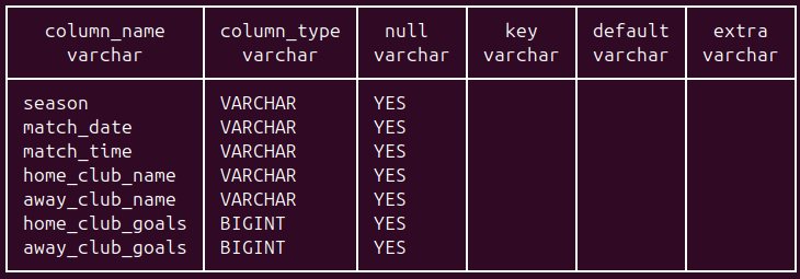
The column names we added in our processing shell script were correctly used by DuckDB as table column names. The column types are more interesting; it has assigned type VARCHAR to five of the seven columns. DuckDB’s VARCHAR type behaves like the TEXT type in PostgreSQL which is convenient because it does not requires a length value as it does in many other database software where you need type declarations like VARCHAR(50). It is also a general data type that can represent date values or numbers as text that can be converted to more appropriate types as needed. For example, we have a date column but DuckDB has interpreted the date strings as VARCHAR and has not tried to be “clever” like Excel and do automatic type conversions! It has inferred a type of BIGINT for the columns home_club_goals and away_club_goals. DuckDB has many numeric types and it has correctly inferred an integer type for these columns; it has “played safe” by assigning the biggest integer type but common sense tells us no football score is ever going to need such large integers as this type allows. We will cast these columns to a more suitable integer type later.
Tip:It is always worth checking carefully what types DuckDB has inferred because if you expect a numeric type for a column and it assings a character type, then it may indicate mixed data types in the column or that the columns are not aligned correctly.
Loading season 1992_1993 data
We only have a Wikipedia crosstab table version of the match scores for this season. For now, we will just import into the staging schema.
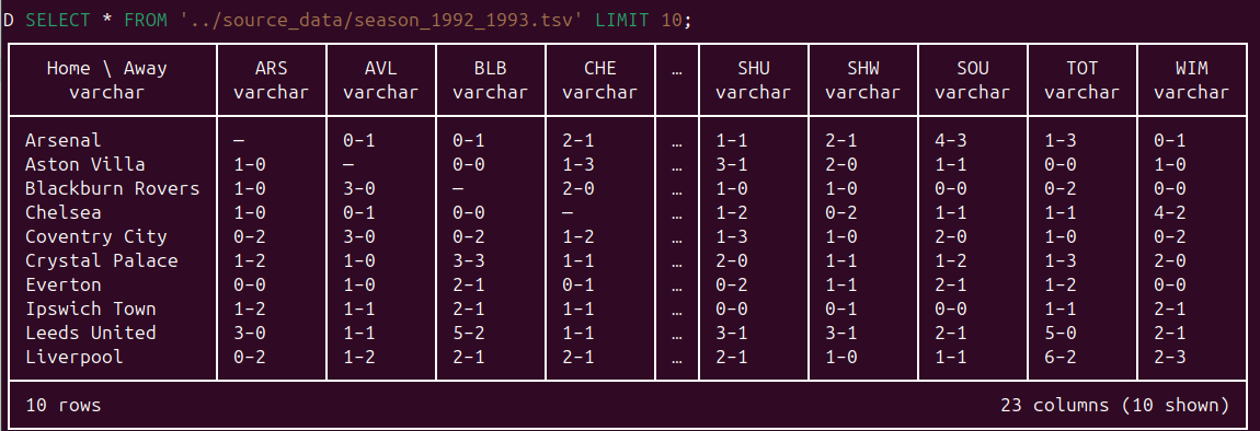
Let’s first take a look at the first 10 rows:
SELECT *
FROM '../source_data/season_1992_1993.tsv'
LIMIT 10;
This shows us the first 10 rows and confirms that we have the expected 23 columns, as show below:
 _
We can now import the table and get to work extracting its data into a more usable format.
_
We can now import the table and get to work extracting its data into a more usable format.
USE SCHEMA staging;
CREATE TABLE season_1992_1993_raw AS
SELECT *
FROM '../source_data/season_1992_1993.tsv';
Re-formatting this dataset to make it compatible with the other seasons’ data will be an interesting challenge and a chance to practice with DuckDB’s very powerful UNPIVOT SQL command.
Main points
- Discussed the two types of commands that you can execute in the DuckDB client
- Dot commands
- SQL commands
- Created the following DuckDB objects
- A DuckDB database - epl.ddb
- A schema within the database - staging
- Created a new DuckDB table seasons_1993_2023_raw in the schema new schema
- Verified that both data row counts and the number of columns in the new table were as expected
- Used the DESCRIBE command to get a convenient view of the table column names and data types.
Next steps
The data we need is now in DuckDB but we need to:
- Verify it.
- Convert columns the right data types - dates, for example, are stored as strings and need to be converted.
- Re-shape the crosstabbed 1992-1993 season’s data to make it consistent with other seasons’ data.
- These analysis-ready tables will be created in the main schema.